Prelab

Sending and Receiving Data

As with the previous lab, I plan to have two separate system states: Collecting Data and Transmitting Data. In the first state I also have my control loop. This way, I first collect data while controlling my car, then I stop my car and transmit the data to my laptop for analysis.

To maximize my data rates, I fill up my characteristic array full of data before sending. I've seen some projects projects upload one data sample per characteristic array, but I tested in lab 1 that I can only send characteristic arrays at around 42 Hz, which makes my payload rate my limiting factor. Therefore, if I can make my payloads larger, I can send data faster.

The code to set this up is quite easy:

Serial.println("Finished collecting data. Sending now.");

int count = 0;
while (count < data_length) {
    tx_estring_value.clear();
    while ((tx_estring_value.get_length() < 100) && (count < data_length)) {
    tx_estring_value.append(timesIMU[count]);
    tx_estring_value.append(",");
    tx_estring_value.append(accelX[count]);
    tx_estring_value.append(",");
    tx_estring_value.append(accelY[count]);
    tx_estring_value.append(",");
    tx_estring_value.append(accelZ[count]);
    
    count++;

    if ((tx_estring_value.get_length() < 99) && (count < data_length)) {
        tx_estring_value.append("|");
    } else {
        break;
    }
    }
    Serial.println(tx_estring_value.c_str());

    tx_characteristic_string.writeValue(tx_estring_value.c_str());
    delay(30);
}

Serial.println("Sending Data Complete.");
                        

I just iterate over my data storage arrays, making sure that I only send the characteristic array over to my PC when it's string length gets close to its maximum value. After sending the characteristic array, I wait a short moment before filling it up and sending it over again.

From my PC's side, I just start my notification handler that parses the c-string that I receive over Bluetooth, and store that data into lists so that I can work with them in Python.

Lab 5

ToF Sensor Data Rate

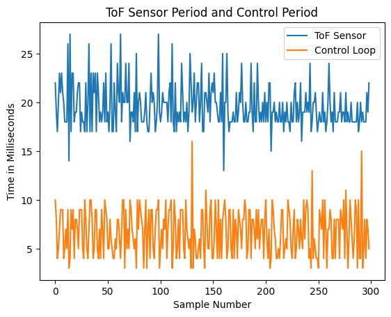
After pulling a few hundred data points from the ToF sensor, I plotted the time between samples, and found that the average sampling rate is around 40 Hz, and it's consistent. I'm happy running my control loop at this rate. I think that sometimes, this rate is limited by compute efficiency, not the sampling rate of the sensor, so if I optimize my code, then I can probably bring in the upper limit of sample periods from 30 ms down to around 20 ms.

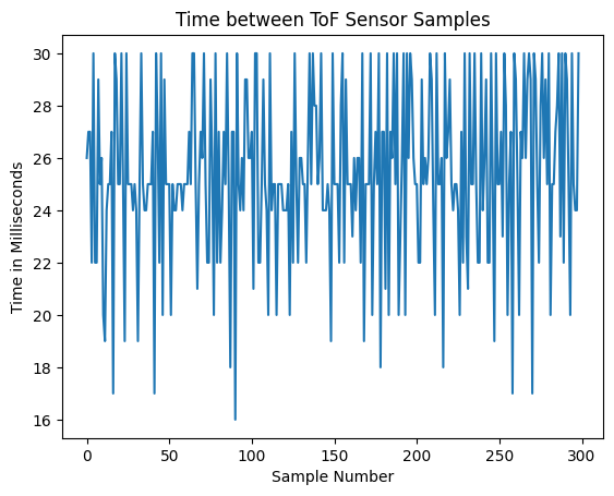
It's just a happy coincidence though that my PID control loop is running around the same speed as my sensor speed. In the future, I'll add more processing-heavy algorithms and also optimize my code heavily so that my control loop can be super fast, so I'll want to decouple these two rates from each other.

Extrapolation

Since I'm going to control at a faster rate than I can get data from my ToF sensor, I'm going to need to extrapolate my data. To do so, I'm going to use the slope of my ToF data, and project that slope from my most recent data point to get an estimate of where I am. Unfortunately, my ToF sensor data is really noisy, and differentiating a noisy signal makes it garbage. So I put a first-order LPF on the differential input, and also put more filtering on the output.

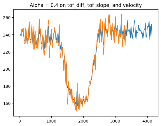
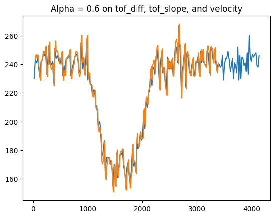
alpha = 0.4 wasn't good enough, so I increased it to 0.6, and I was happier with my results, but after looking closer my values, I realized I had a lot more phase margin to take advantage of. Here's the plot of alpha = 0.6:

After zooming in, I could see that I could afford to make my differential much more filtered.

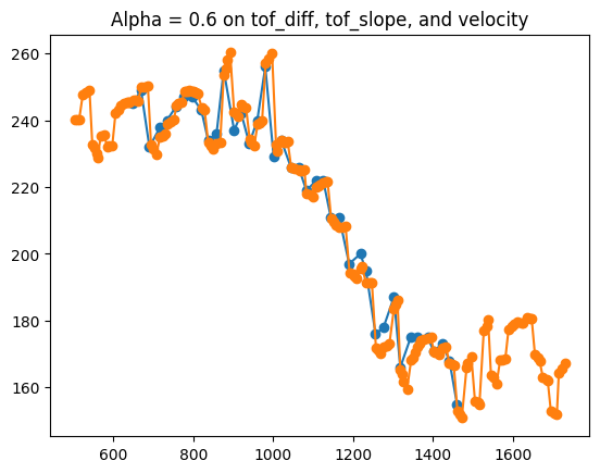
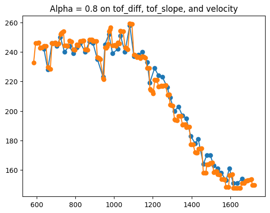
So, I increased my alpha to 0.8, meaning that 80% of my next data point will depend on past data.

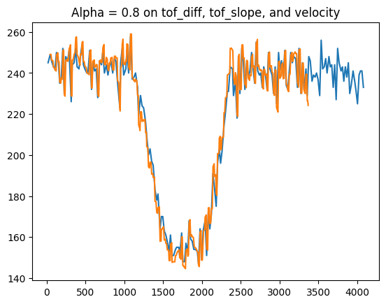
If you zoom in on the data, you can see clearly that the filter is working well to yield high-quality, extrapolated data.

In addition, my control loop is now running a lot faster because I got rid of print statements. My control loop runs 3-4x faster than my sensor.

By the way, in testing, I found that updating IMU data takes about 4 ms alone. That's really long.

The fact that my control loop is running 3-4x faster than my data acquisition time means that extrapolation can make a significant difference in the quality of my control here. My P controller might be a little more jerky without good extrapolation. I would also build up my integral term faster because I'm collecting more error.

PID Control

For feedback control, I started with a simple P controller. This kind of worked, but I felt it was too slow, so I decided to add an integral term. Unfortunately, after tuning for a while, my car kept overshooting even as I turned k_i smaller and smaller. Eventually it was basically zero (0.00002), so I decided to try adding a derivative term to cancel out the integral windup. This caused the car to get really jerky, and I kept on getting weird spikes in the billions, which is really bad. I'm sure this was a fixable problem, but the other solution was to just go with a P controller again and make it work rather than have an "optimized" system that doesn't work. So, I went with a P controller and used a really low saturation value for my control signal so that I wouldn't overshoot.

This worked really well. In hindsight, it was pretty dumb to use a PI controller here since I don't have any forces acting on my car. It's perfectly semi-stable, so I really don't need the integral. I PD controller might work well here, if I can get the derivative portion to stop spazzing out.

I think later on I'll try to get a PD controller tuned to hell and not worry about the integral term. It would be cool if I could get the car's wheels to turn backwards while slowing down. At the end of the day, I made the car work with kp = 0.05, ki = 0.0, and kd = 0.0.

Range and Sampling Time

I think the range of the sensor really doesn't matter much here. When the car is over 1.3m away, the control signal is probably saturated anyways, so it really doesn't matter if you're 1.5 m or 2 m away from the wall, you're just going to accelerate at the wall anyways. In terms of precision, short range mode might help marginally here, but I still don't think it's that big of a deal until you get a pretty aggressive derivative term.

As for sampling time, my ToF sensor runs at around 40-50 Hz, and my control loop is running at around 100-150 Hz. This is why extrapolation of my ToF sensor data is important.

The road to feedback control

I started this lab in a really dumb way. I thought that it'd be cool to not only extrapolate data, but use a complementary filter to combine IMU data with ToF data. This was a terrible idea because my IMU gave me so much drift that I thought it was an issue with how I was calculating my values. So I was "debugging" an intrinsic problem with my system for like six hours.

After realizing my mistake, accepting failure, and deleting all my code, attempt 2 was a little smoother. Extrapolating the pure ToF sensor data went pretty smoothly, although I needed to use a much stronger LPF than I anticipated. I guess this makes sense because you're differentiating a noisy signal, and that usually gives you garbage, but I didn't internalize the extent of that at first.

I spent a while tuning three LPFs that I put in my data acquisition system. One of the LPFs was on the differential data[n-1] - data[n-2]. The other two LPFs were cascaded on each other on the differential output. This gave me a second-order LPF that worked really well to prevent spikes in the raw data from affecting my extrapolation.

I made sure that my ToF sensor was really high quality because I knew from experience that feedback control tuning gets really easy if you have good data and good state estimation. So from here, things went pretty smoothly.

As mentioned before, I started with a P controller but was unhappy with its slow performance. So I moved on to a PI controller, which gave me overshoot, and then I added a D term to compensate for the overshoot. This didn't work because I got a ton of noise on my D term, so I spent some time thinking and realized that this system doesn't even need an I term at all. This is because there are no constant forces like gravity here. The entire car's state space is semi-stable, so an I term just adds either oscillation or overshoot. Either way it's eating up my phase margin. I've also tuned my car's movement so that there's no "threshold" level of throttle for the car to move. move(255) is really fast and move(1) is really slow, but the car is only still when I write move(0).

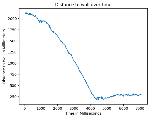
Anyways, by switching back to a P controller, the system worked really well and the car stopped right at the 12 inch mark from the wall, which is great. Here's a video of that happening:

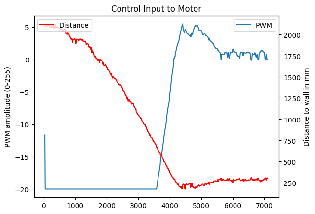
And here's a graph of the position from the wall over time. You can see that it spends most of its time in saturation, and it has a small overshoot due to the momentum of the car as it approaches the setpoint:

You can also see more definitely that the car spends most of its time in saturation by looking directly at the control input to the motors. Here's a graph of the PWM amplitude over time:

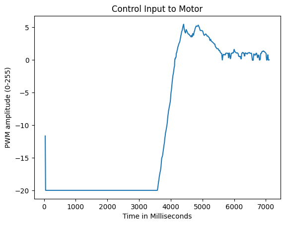
If we put the two graphs together, you can see how the control signal saturates in large error and how it reacts to in the actual position as you overshoot and come into the steady-state position:

Conclusion

Overall, I learned from this lab the importance of good data in control systems. It's an information problem, so if you have bad info, you'll have bad control. Also, I learned the simpler is better, and that it's worth it to build systems step-by-step instead of all at once, especially for algorithm-based programming like this. I'm also glad I put effort into making my car robust, because I didn't have to worry about it failing at all this lab. I'm looking forward to implementing better state estimation techniques like Kalman filtering in future labs and using that to make better control systems.