Prelab

PID Input Signal

The name of the game here is high quality orientation data. My IMU measures angular velocities in the directions of roll, pitch, and yaw, which means to get actual position, I need to integrate my values. This can cause some pretty bad drift over time.

One way I can minimize drift in my orientation data is by using arctangents of my IMU's accelerometer to find absolute position. The issue with this data alone is that it doesn't give me yaw, and it also gets unusably noisy when either the x or y components are near 0. So to compensate in these regions, I can rely more heavily on the gyroscope data.

In terms of sensor limitations, the ICM-20948 is a very capable sensor, but it does have a maximum degrees per second of rotation that it can measure. Similarly, it also has maximum acceleration and magnetic amplitude, but I think the rotational acceleration is going to be the first maximum that I hit, if I do. According to the ICM-20948's register mappings, the default gyroscope maximum degrees-per-second is +- 1000, which is around 3 revolutions per second. This should be sufficient for me, and I'll keep in mind not to go over this limit in my testing.

Sending and Receiving Data

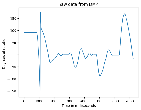
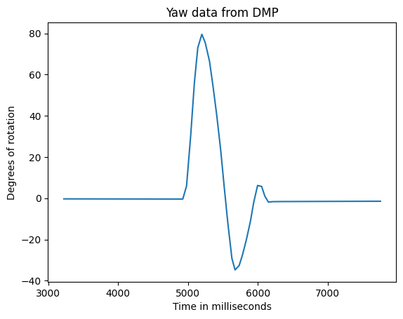
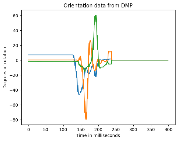
As I said before, with controls, high-quality data is key. The better your data is, the better the control. So, I need to be able to collect data from my Artemis, and send it to my PC for analysis. To do so, I used the example code from the ICM-20948 library to set up my DMP. After some basic functionality testing, I checked that the data I recieved to my PC matched what I expected based on the car's movement.

Once I was happy with the DMP data that I was collecting, I moved on to retuning my move() function. This function would take in a value between -255 and 255, and it would make the car rotate at a certain rate. Unfortunately, the static friction to overcome rotation is much higher than the static friction to overcome rolling forwards and backwards, so I had to retune my move() function. I did this using a temporary command over ble that would allow me to remotely change my tuning values:

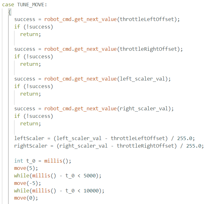
This allowed me to rapidly find my offsets and scaling values for my left and right motors so that the robot would spin well in one spot.

Lab 6

PID

The PID loop that I wrote worked well to control my robot's yaw, but the integral term was almost zero in my final tune. My final values were Kp = 0.4, Ki = 0.002, and Kd = 0.05. This gave me good damping near my setpoint, and high acceleration when I was far away from my setpoint. The fact that Ki was so small reinforced my theory from Lab 5 that for a semistable system such as a car on flat ground, the integral term is simply unneeded. It only really causes overshoot and phase lag. Again, for the final tune in later labs, I'm going to go with an optimized PD controller because I think that will result in the best performance for my system. Here's a video of my controller operating:

Sampling Times

Since I'm no longer polling my time-of-flight sensor, my control loop has drastically sped up. Here's a histogram of the number of milliseconds that each control loop takes:

As you can see, the time between controls is drastically shortened compared to the 15-25 milliseconds that a control loop in Lab 5 would take. This is because I optimized my code by removing unneeded low pass filters. I could do this because the data that a got from the DMP was a lot less noisy than the data from the time-of-flight sensors.

This ensures that my control rate is at least 10x faster than the dynamics of my system.

Development Process

As previously said, my first goal was to acquire high quality data from the DMP, so I used the example code provided by the library to play with my car's Euler angles and orientation. Once I found that I had low-noise, high accuracy orientation data that didn't drift over time, I integrated the setup() code into my own bluetooth program, and reported that DMP data to my PC over Bluetooth.

Once I observed this high quality data streaming to my PC, I had the confidence to employ the PID code from lab 5. This was mostly just copy and paste, since my control code was fairly functional. I was also able to remove a lot of complexity because I no longer needed low pass filters for noisy data and clamping because I tuned my move() function much better this time around.

High quality data and good actuators made tuning my PID loop very easy. I used a simply Zeigler Nichols approach, increasing Kp until I saw a lot of oscillation. This indicated that I was at the edge of stability. I then started with 0.6 Kp, 0.5 Ki, and 0.125 Kd, but this worked poorly. I knew that the integral term was the source of most of my problems because I was in a semistable system, so I reduced my Ki term and increased my Kp term. I knew I was going in the right direction because my controller quicky got much faster and less oscillatory.

Here is a plot of my yaw data over time as I kick the car once. You can see that it deflects almost 90 degrees, but it is able to recover quickly with limited overshoot. My setpoint in this example is 0 degrees.