Estimate Drag and Momentum

Steady State Velocity

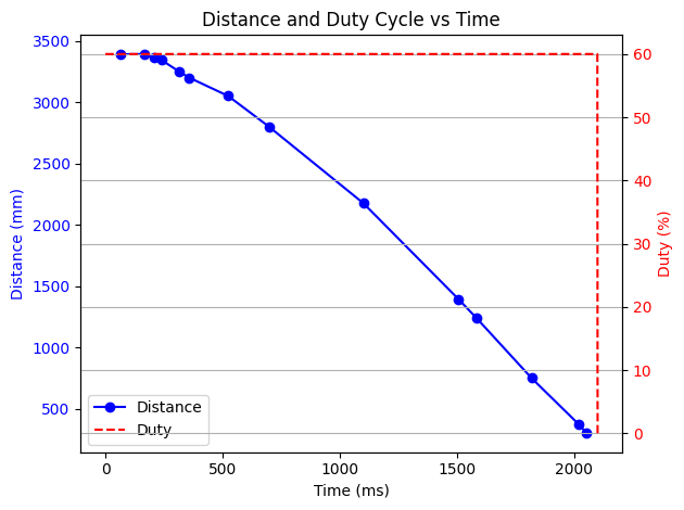
Prior to writing the Kalman Filter, I need to characterize the dynamics of my system. I need to calculate the drag of my system. In order to do this, I need to find the steady state velocity of my system. The steady-state velocity was defined as the velocity when I send a PWM duty cycle of 150 into the motor drivers. This is roughly 60% duty cycle. I then measured the position of the car from the wall using the time-of-flight sensors, and I recorded the time of each measurement. Using this data, I calculated my steady-state velocity.

From the chart you can see that the car is moving at a constant velocity toward the wall. Then it hits 0 distance which means the car impacted the wall. At the same time, I cut out the command to the motors. After that, it spins a little and then settles down.

If I take the window of data only when the car is moving at steady state velocity, I get a nice, linear plot of the distance as the car approaches the wall at a constant speed. Unfortunately the time-of-flight sensor doesn't take data points very often, but the data that it does collect is quite high-quality.

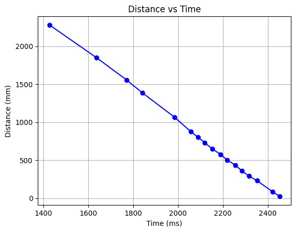
Using the gradient() method in numpy, I calculated the velocity of my car at each time step. I then took the average of these velocities to find my steady-state velocity.

I found that the steady-state velocity of my car at 60% duty cycle was 2.1 m/s.

Rise Time

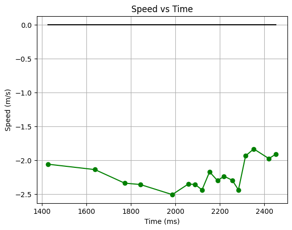
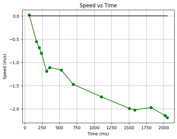
Now that I know my steady state velocity, I can find my rise time, the time it takes to get to 90% of my steady state velocity. I can do this by accelerating my car from 0 speed up to steady state velocity, and measuring the time it takes to get to 90% of that speed.

If I graph my velocity, I can see that it takes about 1500 ms to get to my 90% steady state velocity.

Drag and Momentum

I can use my equations of motion to get expressions to calculate my drag and momentum. Here are my A and B matrices:

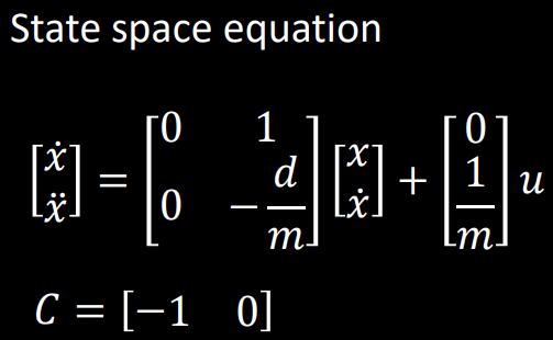
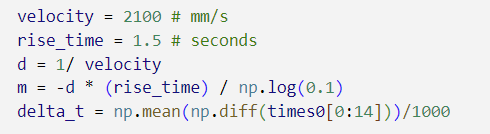
According to this system, drag will be 1/steady_state_velocity and momentum will be -drag*rise_time/ln(0.1). This math is done in the python code below:

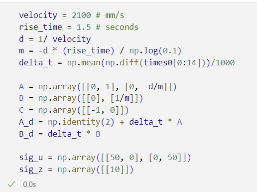
Kalman Filtering in Python

Using my empirical values for drag and momentum, I can create my A, B, and C arrays. I took the average time between samples during my max speed run, and used that as my sampling period. I could see an issue with the Kalman Filter and the time-of-flight sensor because of the high variance of sampling time, but the Kalman filter should be able to compensate for that if I tune my data vs prediction covariance matrices correctly. I put values of 50 to fill sigma_u after tuning the process noise to get good results for the acceleration test case. I also used a value of 10 for sigma_z, which is the measurement noise covariance matrix. This is because I know that the time-of-flight sensor doesn't have that much noise in its measurement. I started with a sigma_3 value of 50, but found that this was too high, which is how I ended up with a value of 10 for sigma_z.

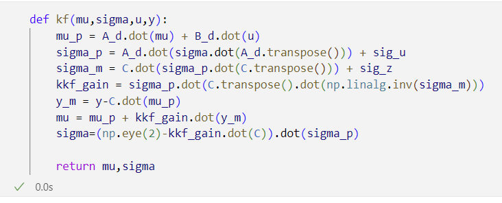
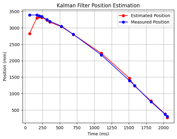
I then wrote the Kalman Filter estimation step in python, as well as a loop to test the Kalman filter's ability to estimate the state of my car.

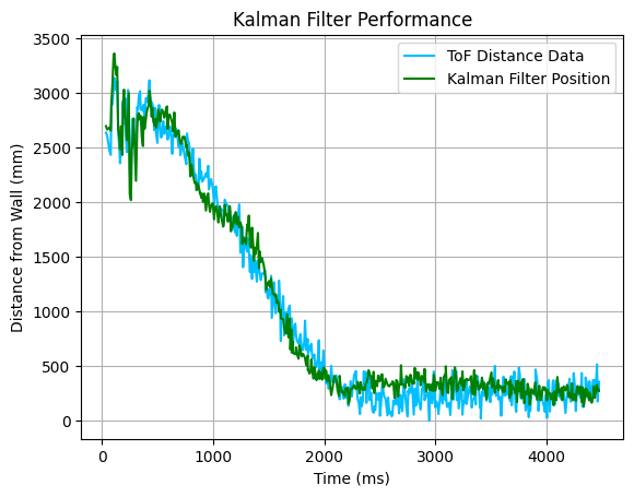
Kalman Filtering on the Car

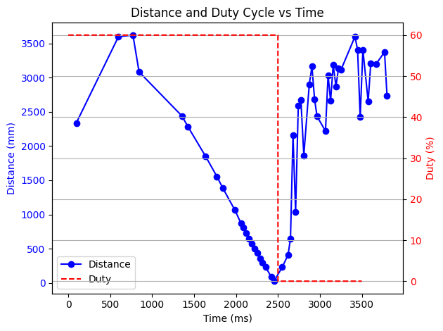
Instead of reading from my interpolation algorithm from Lab 5, I used the Kalman Filter to estimate the position of my car. This didn't increase my rate of data like the interpolation did, but it made my data a little less noisy without introducing phase lag. While I was here, I also made my PID far more robust, and got the car tuned really well.

Using the Kalman filter and improved PID, I was able to control from a much farther distance, and I was able to raise my clamps by a lot. This meant that I approached the wall much much faster, and I'm really happy with the performance of my system now.

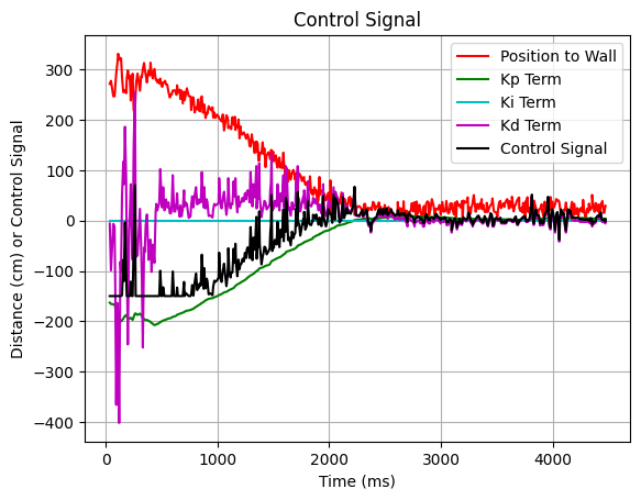
Here's a graph of my PID values over time as I approach the wall: